Audio: Lemmings (vidogame) Soundtrack - Stage Theme 6 by Brian Johnston and Tim Wright.

One of the more challenging topics for students in 1st year biology courses is evolution. Introduction to Evolutionary Biology A difficulty in understanding evolution is that it is a process as compared to a bunch of moving parts for example translation or protein structure. Another aspect of the challenge is that most of the important lines of evidence for evolution (homologous fossil structures, cytochrome c sequence cladistics, biogeography, etc) require inferring how those support common ancestry. Namely, one can rarely directly compare two related species to a living example of the common ancestor.

Two other major fields of study have been important for understanding evolutionary processes: Genetics and Ecology. Mendel's Principles of Inheritance described genes and how they are passed along and a useful nomenclature for describing inheritance and physical characteristics of organisms. His selected traits also followed predictable probabilities which specifically describe the segregation of chromosomes during meiosis. Although, his principles apply to only a small set of actual inheritance patterns (only two variations (alleles) of a gene with expression of only two types of phenotypes), they are really useful and are fundamental in 1st year biology courses.

The study of populations of organisms and how they vary numerically over time has influenced how one teaches evolutionary concepts as well. While primarily limited to the realm of microevolution, the advantage of a description of changes over time help visualize the evolutionary process related to the selective pressure.

The Hardy-Weinberg equation is a marriage of the last two concepts that describes allele and phenotype frequencies in a population over time. Under nonselective conditions (each individual has the same change of survival), the frequencies do not change much in large populations. However when allele frequencies are seen to change or genotype frequencies break from the expected, it is suggestive of a selective process favoring one of the two alleles of the gene. Thus, analyses of simulated or real populations using Hardy-Weinberg are useful for understanding evolution. The problem with this approach is that it typically involves math, another bane of teaching 1st year biology students, in particular non-science majors.

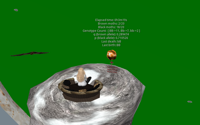
This virtual Population Genetics and Selection activity is designed to give students the opportunity to observe a population of organisms experiencing a selective pressure and observe changes in the genotypes and phenotypes over time. There are two important components as a learning exercise fitting with the objectives of the BIO-SE group:

1. mimicking the mathematics of population genetics and inheritance and
2. providing a visualization of the evolution process that is flexible in terms of the examples employed
3. the ability of the student to interact and generate data with variable user input to feel a sense of engagement and ownership

The initial example used and described here is from the classic example of moth populations in England. A recent paper has identified the gene involved ¹⁾ and a review in Nature gives a good overview The peppered moth's dark genetic past revealed In brief, the peppered moth in Britain (Biston betularia) was found to be predominantly a light brown color in the middle 1800s but included darker (black) individuals. The light brown coloration relatively well matched the predominant tree bark color and helped with survival against predation by birds. With the industrial revolution and it's associated fossil fuel burning, a significant amount of soot accumulated on trees such that light brown no longer blended as well and the black moths did. This led to a documented increase in the percentage of black moths in that population.

Another good example of this type of selection is found with mouse coat colors which I first stumbled upon from NOVA's What Darwin Never Knew.

• Coloration is the trait for moths and can be either brown or black
• B is the allele for black
• b is the allele for brown
• as denoted by convention the capitalized allele is dominant which means in a given moth that has 2 alleles Bb will be black (BB is black and bb is brown)

• p is the frequency of B in any given population (it is also the probability that any given allele in an organism will be B)
• q is the frequency of b in that same population (it is also the probability that any given allele in an organism will be b) because there are only two choices,
• individual alleles contained in gametes are passed from parents to offspring (one from each parent so a total of two in any offspring). The selection of which gamete from a parent will generally be considered random, then the frequencies of BB moths, Bb moths, and bb moths in the population will be represented :

a nice short description of this is found here

• a starting population of moths with the appropriate allele frequencies (set by user input, default p = .5) and visually represented corresponding phenotypes (B and b alleles, black (BB/Bb/bB) or brown (bb) coloration
• a selective pressure that leads to "death" of individuals in the population (predation by bats ²⁾)
• the selective pressure is exerted by having the two populations coexist in a given space with theoretically random movement (see Wanderer script) and to allow Second Life "collisions" to represent an encounter between the two.
• an environmental variable in which "death" is equally probable between all phenotypes (lichen covered or "green" tree trunks has 80% death for any moth when it and a bat undergoes a virtual world collision)
• one or two environmental conditions in which there are differences in the death probabilities for the different phenotypes ("sooty" sphere (to represent coal covered tree trunks) changes probability of death for black moths to 20%, brown bark changes probability of death for tan moths to 20%)
• the ability to detect a death and input a replacement into the environment to keep population size constant (really important aspect of this simulation is that it will also count the current live specimens to determine p and q at that time and create a new moth with a genotype based on the current population allele frequencies)

While actual activities, worksheets, demonstrations, and assignments can be designed in different situations in mind. The hope would be that over the course of a few days students could have their own object that they rez and set different parameters to observe the changes and quantify allele and phenotype frequencies over time. So for short demonstrations setting the number of starting moths really high and setting p in a way that has a small number of the advantageous phenotype to start and having lots of predators would be optimal. However, in assignments for students one can explore several scenarios that take longer or go through several iterations (like starting multiple times with very low numbers of moths like 4).

This current design is to allow students to visualize and explore the basic Hardy-Weinberg concepts of allele and phenotype frequencies over time due to simple predation. The input variables of environment, p, and population size are sufficient for these purposes and can help demonstrate genetic drift (using small populations).

Future capabilities to explore more aspects of population genetics can be built upon this foundation. Some initial ideas include: # because of the flexibility of the Wanderer scripts capabilities one can mimic different predator/prey examples. Bats and moths both fly in spheres but other examples could include: sharks attacking dolphins with white ventral coloration or not from below, different fish colorations, cats could have overlapping disk with mice, or owls could descend from above on mice, etc. # because genotypes are tracked within mice, one could have replacement mice come from collision events between mice to represent mating events # inclusion of gender, more genes, or nonMendelian inheritance patterns (co-dominance, partial dominance, sex-linked, etc) to represent how inheritance patterns might affect selection power. # the ability to change the population size and selection environment mid-simulation to demonstrate bottleneck affects and to allow nonselective breeding after selection which will allow larger data sets to equilibrate to Hardy-Weinberg conditions # the ability to insert individuals with different p and q to demonstrate founder effect and gene flow (migration).

The Population Genetics and Selection (PGS) simulator is a rather complicated build because of the different pieces of information that must be exchanged between the PGS, the birds of prey, the mice and the statistics/allele tracker. In total, the PGS uses 3 (cleverly) shared channels as well as link messages in order to provide some synchronization between the various components.

First, the birds of prey and the mice are individual objects using physics for collisions to simulate death. For the mice, llVolumeDetect has been used, making the mice phantom yet still subscribing to collision events so that the mice are not affected by collisions amongst themselves or with avatars but rather exclusively with the birds of prey.

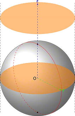
For the general motion, we used the Wanderer script which provides an elegant way to move the mice and the birds of prey independently. The birds of prey move by selecting points in an upper hemisphere and the mice move by selecting points inside a circle. One elegant consequence thereof is that the volume of the area defined by the upper hemisphere and the area defined by the points inside a circle intersect in the lower part of the hemisphere offering the circle cross-section that generates our collision events leading to the consumption of mice by the birds of prey (Figure 1).

Every mouse has an associated genotype which can either be BB,Bb,bB for brown mice and bb for black mice.

We define the P-probabilities of both possible alleles B and b as:

and

When such diploid organisms reproduce, they make sex cells containing a single copy of each chromosome in a fifty-fifty percent ratio. Thus, fifty percent from a Bb mouse will contain the B allele and the other half will contain the b allele. Each parent donates one sex cell, resulting in an embryo with two copies of each chromosome, one from each parent. For example, two Bb mice would have a 25% chance of producing a BB offspring, a 25% chance of producing a bb mouse and a 50% chance of producing a BB offspring.

Under the theoretical assumptions made by G. H. Hardy and W. Weinberg in 1908, we have the following genotype frequencies:

Since we have the extra condition that:

since the probabilities are complementary, we can check whether:

Using p-q probabilities, and since we know that P(Bb) = P(bB) = pq, we can re-write the equation:

Which is a second order quadratic equation, the roots of the equation being:

we additionally know that:

so we substitute (2) in the first equation (1) and obtain:

Now, we know from the polynomial expansion rule that:

and we use the rule (4) in our substituted equation (3):

simplifying (5) and discarding the negative probability root, we obtain that:

Which shows that the probability equation always checks out for a given p and a derived q (taken as ).

The PGS uses two types of movements, based on an optimized version of the Wanderer: movement within a circle and movement within a sphere. We describe both of them below, pointing out how the coordinates are generated.

So you find yourself on a desert island and you want to be rescued. You plan to write a huge SOS in the sand so air traffic may spot you. How would you draw the O in the sand so it is a perfect O? (How about the S?).

Since the dawn of time, people have been using compasses (Figure 2) to draw perfect circles. It works on a simple principle, you select a starting coordinate (called the origin O) with the sharp point of the compass legs and then you move the other leg around which usually contains a graphite tip. Since you have a fixed point, and a radius (the distance between the two legs), when the graphite scratches the surface of the paper, it sketches a circle.

In our application, one of the movements is a movement inside a circle starting at an origin point (O) and having the radius you define in the header of Wanderer. If you look at the video, that origin point is the very centre of the dome.

Thus, we need to generate points inside a circular surface which will be our next coordinate that our creatures will travel to. Since every creature has a Wanderer script, every creature will move independently by generating its own set of coordinates within the circle bounded by the dome terrain.

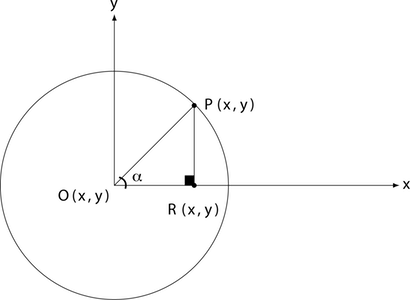
To do that, let us take a look at Figure 3. We have the origin point O with the coordinate pair (x,y), similar to the sharp point of the compass in an x-y cartesian system. The segment OP is the radius, it goes from the origin point of the circle O and to a point P on the circumference. Additionally, we have another segment PR which is just a projection of the point P on the Ox axis.

If you look at Figure 3, the square blackened rectangle shows you that this triangle is a right-angle triangle which allows us to use some trigonometry.

We know that:

Let us substitute OP with r, because we know that OP is the radius of the circle. Furthermore, let us substitute PR with y and OR with x since we know that those segments represent the distance from the origin point O to the point P. Now, let us write the equations again:

Now, we solve for x and y:

What we have obtained is the parametric from of the circle equation.

How does that help us? Well, suppose we want to pick an arbitrary point G within the circle. All we have to do is to choose the angle α and a radius r and then calculate x and y. Our point G will find itself at the coordinate pair (x,y).

Not sure about that? Think about it, the radius (like stretching the legs of the compass) gives you the distance from the origin point O. The angle gives you the rotation: for example, in Figure 3 the point P is at 45° from the x-axis. The bigger you make the angle, the more P will move on the circumference of the circle to the left (counter-clockwise).

So, let us see how we will do this in LSL. The following is a standard LSL vector, component x and y are exactly what we obtained as the parametric equation of the circle earlier.

<r * llCos(α), r * llSin(α), 0>;

If you keep choosing a radius r and an angle , you will obtain different vectors describing positions inside a circle area. As you can see the z-component is set to zero so that we do not generate points within a cylinder (can you see that?).

The problem though, is that if you do that for a region and you use region coordinates, you will of course generate points at the very corner of the region because the origin point O has the coordinate pair (0,0) - that is, on a region the coordinate (0,0) finds itself in the corner of the region.

In order to avoid that, we must offset this origin point O. We must move it from the corner of the region to somewhere more useful. We simply apply an offset we want to both x and y components of the parametric form of the circle equation:

Going back to LSL:

<offsetX + r * llCos(α), offsetY + r * llSin(α), 0>;

That is how the points are generated within a circle by Wanderer. When the PGS simulation starts, it records that offsetX and offsetY with llGetPos. Since the scripts are within a sphere, llGetPos will give us the offsetX and offsetY that we need so that the origin point of all wandering creatures is right in the middle of the sphere. Now, you can take a look again at Figure 1 and observe that the shaded circle is right in the middle of the sphere, the mice moving inside that circle. They do that by selecting a random radius (within bounds of the dome) and a random angle and then moving to the point described by those parameters using llMoveToTarget.

As for the S question, you keep the compass in the same coordinate and you draw two symmetric semi-circles in opposite directions. One S-hook is really a semi-circle.

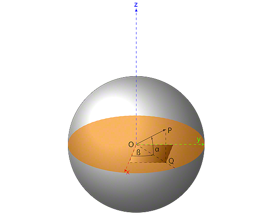
A sphere is a generalization of a circle on in an x,y,z cartesian axis-system; in other words, a generalized form of a circle in 3D instead of 2D. In order to deduce the equations for a sphere, we refer to Figure 4.

The segment is created b the projection of P on and is also the bisection of the rectangle described by . is a perpendicular projection on the x-axis and is a perpendicular projection on the -axis.

In the triangle between and the x-axis:

In the triangle between and the y-axis:

In the triangle given by :

Now, we take the last equation:

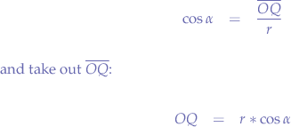
and substitute in the first two equations:

we extract x and y since it is what we are looking for:

we also need z, so we go back to the triangle :

so we extract z:

Now, concluding, we obtain:

which is the parametric form of the equation of a sphere in space. If you follow what we did, we really did the same thing that we did for a sphere, but we just did it several times in order to obtain z as well.

Of course, we should add an (optional) offset, just like in the circle case, since we do not want a sphere at the region corner:

Since we have obtained the equations for our sphere, we can now just chose a random , such that:

and also a random radius r, such that:

In LSL, from Wanderer we can now write the LSL lines that will generate our random spherical points:

float α = llFrand(TWO_PI);
float ß = llFrand(TWO_PI);
float r = llFrand(MAX_RANGE);
vector P = llGetPos() + <r * llCos(α) * llCos(ß), r * llCos(α) * llSin(ß), r * llSin(α)>;

The vector P, a point-vector, will be a point within a sphere described by the arbitrary angles , and arbitrary r and starting at the position where the calculations are performed (llGetPos).

Depending on the uniformity of the random number generator that we use to pick , and the radius, the generated points will have different overall distributions in space.

Now that we know the parametric equations for a sphere, we can determine what we have to do in order to get a hemisphere. A hemisphere is half a sphere however, if you look at Figure 4, you could have an upper hemisphere and a lower hemisphere: a bit like cutting an orange.

Let us look at the sphere equations again:

Now, when we cut, we want to slice the sphere in half on the z-axis (however, you may just as well cut on any other axis). So let us look at the z-point equation:

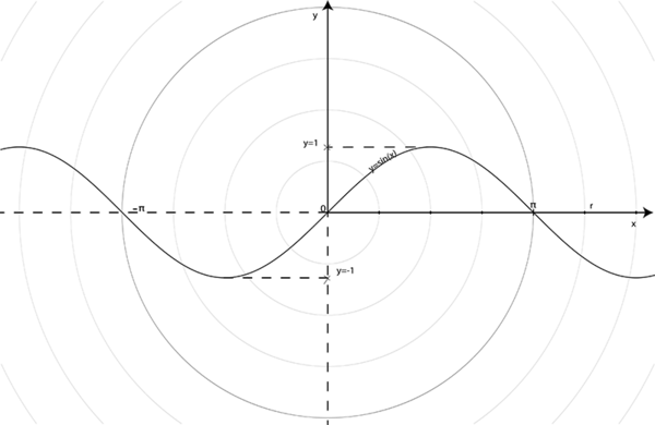
And let us see how this works: sine is an alternating mathematical function. That is, you take a value for and will be a value in the continuous interval [-1, 1]. In Figure 5. we represent the sine function , using a radial grid and a radius of an arbitrary circle, with .

That means, whatever I feed as to , we will obtain a value between -1 and 1 (inclusive). However, we know know that our algorithm generates the point z using:

If you look at Figure 5, returns a positive value for the interval (0, PI). Thus, the simple way is to take our former equations:

We have to make sure that is a value between 0 and , whereas can be a value between 0 and 2*PI. In fact, if you go to our sphere figure, Figure 4, you will see that the angle gives us a rotation around the z-axis, whereas gives us a rotation around the x,y-plane.

Written in LSL, we have the code we used before, except that α is a random angle in the [0, PI) interval:

float α = llFrand(PI);
float ß = llFrand(TWO_PI);
float r = llFrand(MAX_RANGE);
vector P = llGetPos() + <r * llCos(α) * llCos(ß), r * llCos(α) * llSin(ß), r * llSin(α)>;

which will give us a movement in the upper hemisphere. Symmetrically, we could restrict α to be a value in the interval (-PI, 0] for a lower hemisphere.

To be complete and end the discussion roundly, you can take the same trick and apply it to the circle equations to get a semi-circle. However, since our PGS uses either circular or hemisphere movement, these are sufficient.

Newtonian physics, mechanics teaches us that in a gravitational field, every object is susceptible to gravity. Once you subscribe to the physics engine by setting status to true, with:

        llSetStatus(STATUS_PHYSICS, TRUE);

the object will experience a downward force, making it fall down to the ground.

The gravitational force, is given by:

where m is the mass of the object and g the gravitational acceleration, supposing that:

where » stands for much greater than and M is the mass of the planet attracting the object. Sometimes F is noted G to distinguish it from other forces. However, we preferred to just use a generic force letter to eliminate the confusion between G and g.

To deduce this, we take Newton's law of universal gravitation:

and we apply since, in this case :

and then since compared to the distance between M and other planets, r is extremely small (we don't even have any other extremely large masses such as planets in Second Life - imagine Second Life if Second Life would also have different planets, ha! Now that's a dream…) and obtaining:

with k = g = 9.81 in Earth's and Second Life's case.

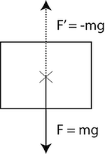
In Figure 6, we can see a force-vector F pushing an object downward. In order to counter that force, we must apply a force-vector oriented exactly in reverse of the downward force and with its scalar value, the same as the original F. In other words, we need to apply -F (Figure 6). Since, in our system, the downward gravity force acts in the negative direction of the z axis, we apply it to the positive direction:

        llSetForce(<0,0,1>*llGetMass()*9.81, TRUE);

where llGetMass returns the mass of an object and 9.81 is the current gravitational acceleration set by Linden.

Putting it together, the following two are sufficient to cancel out the gravitational force:

        llSetStatus(STATUS_PHYSICS, TRUE);
        llSetForce(<0,0,1>*llGetMass()*9.81, TRUE);

For physicists, in Second Life llSetForce is used to start the application of continuous given force. That is very convenient because we can avoid calculating resulting, composed force-vectors from G and the directional force meant to move an object in a certain direction. The reverse, for instantaneous forces, we have llApplyImpulse in LSL terms.

Now, for a proper simulation, the probability p is input by the user at the start of the simulation. By default, without modifying p, the scripts have a default setting of:

p = .5

which, based on the former, allows us to compute the probability table for P(BB), P(Bb), P(bB) and P(bb) in the case of the default setting p=.5 (and derived q, q=(1-.5)=.5):

P(BB) = .25
P(Bb) = .25
P(bB) = .25
P(bb) = .25

which, in this particular case makes the coding of selection easy because all the individual probabilities are identical.

That is, in the case of p=.5 (and derived q, q=(1-.5)=.5) we could declare a list of chromosomes as:

list alleles = [ "BB", "Bb", "bB", "bb" ];

and since the probabilities are identical we could just select one of them, when a mouse is born using llFrand]:

string select = llList2String(alleles, llFrand(4));

However, if we specify a p-probability p=.6 (and derived q, q=(1-.6)=.4), we already have a problem because, intuitively, the individual probabilities of the genotypes will not be identical as in the previous case. Let's see:

P(BB) = .36
P(Bb) = .24
P(bB) = .24
P(bb) = .16

Let us check if we have been consistent and check if the probabilities add up to one: P(BB) + P(Bb) + P(bB) + P(bb) = .36 + .48 + .16 = 1. Which means that the frequency distributions are correct.

In this case, where the probabilities on individual chromosomes are different, we cannot use the previous trick anymore using llFrand and we cannot just select a genotype from the genotype list because we have to mind the individual probabilities of each genotype.

This problem can be solved with some basic statistics: instead of randomly selecting a genotype every time a mouse is born, we generate a random number in the range [0, 1) and compare that to the cumulative probabilities of each element. When we say cumulative probability, we mean the probability of the current element plus the probability of all the elements before. The result of that is that the elements with a lower probability will need a smaller random number but the elements with higher probability will leverage the smaller probabilities in order to have a better chance of getting chosen.

We can express that in LSL easily, using the cumulative probability algorithm:

                list sortedp = dualQuicksort([ llPow(p, 2), p*q, p*q, llPow(q, 2) ], [ "BB", "Bb", "bB", "bb" ]);
                list alleles = llList2ListStrided(llDeleteSubList(sortedp, 0, 0), 0, llGetListLength(sortedp)-1, 2);
                list alleles_prob = llList2ListStrided(sortedp, 0, llGetListLength(sortedp)-1, 2);
                float rnd = llFrand(1);
                float cum = 0;
                string genotype = "";
                integer itra = llGetListLength(alleles);
                do {
                    cum += llList2Float(alleles_prob, itra);
                    if(cum >= rnd) {
                        genotype = llList2String(alleles, itra);
                        jump draw;
                    }
                } while(--itra>=0);
@draw;
               // Got an element and it is now in the variable genotype.

However, for the cumulative probabilities algorithm to work, we must first sort the two lists in descending order: the algorithm must first start off from the smallest probability and keep adding up to the highest one. What we observe is that, Bb and bB are always in order due to the fact that they have the same probabilities so one option would be to simply compare BB and bb and swap them depending on their values. However, for a flexible system, in case at a later point we would like to variate the Bb and bB probabilities, we need an algorithm that can sort these two lists:

                list alleles = [ "BB", "Bb", "bB", "bb" ];
                list alleles_prob = [ llPow(p, 2), p*(1-p), p*(1-p), llPow((1-p), 2) ];

while also keeping the corresponding map between BB and the result of p^2, Bb and p*(1-p), bB and p*(1-p) and bb and (1-p)^2. That is not an easy task but Wizardry and Steamworks has already published a dual-quicksort that allows you to sort a list while maintaining the relative correspondence between them. Our previous algorithm used to sort a list of strings and maintain a map to a list of numbers. However, in this case, we need the reverse of that: we need to sort the probabilities found in the alleles_prob list and maintain the correspondence to the alleles list.

We thus change the algorithm to sort floats (the probabilities in alleles_prob) and maintain the positional mappings to the alleles string list:

list dualQuicksort(list a, list b) {
 
    if(llGetListLength(a) <= 1) return a+b;
 
    float pivot_a = llList2Float(a, llGetListLength(a)/2);
    string pivot_b = llList2String(b, llGetListLength(b)/2);
 
    a = llDeleteSubList(a, llGetListLength(a)/2, llGetListLength(a)/2);
    b = llDeleteSubList(b, llGetListLength(b)/2, llGetListLength(b)/2);
 
    list less = [];
    list less_b = [];
    list more = [];
    list more_b = [];
 
    integer i = 0;
    do {
        if(llList2Float(a, i) > pivot_a) 
        {
            less += llList2List(a, i, i);
            less_b += llList2List(b, i, i);
        }
        else
        {
            more += llList2List(a, i, i);
            more_b += llList2List(b, i, i);
        }
    } while(++i<llGetListLength(a)*2);
 
    return quicksort(less, less_b) + [ pivot_a ] + [ pivot_b ] + quicksort(more, more_b);
}

Now we can modify the algorithm to extract the new sorted alleles while also having the convenience that their associated probabilities are to be found at the same index. This way, every time a genotype is drawn from the list of alleles, the individual probabilities of each genotype will be respected.

• The wanderer script uses trigonometry to generate the next destination for moths and bats. In our final version, we have used the completely uniform distribution of the wanderer algorithm by selecting points instead of using trigonometry.
• In order to make the experiment a challenge, we have eliminated some information off the heads-over statistics. This is meant for exercises with students where they will have to pause the simulation and manually count the moths in order to calculate the p and q themselves.

The current PGS build uses 2 semi-active (intermittently closing and re-opening), shared channels to distribute information from the PGS structure to the birds, mice and the statistics tracker in the middle of the build. The distinction between what type of information is passed on which channels is rather subtle and is mainly meant to avoid collisions as much as possible. Several scripts listen on these channels, certain scripts closing the communication channel, in case they are meant for preliminary configuration at the start of the simulation.

The mice run four threads (scripts), one being a modified version of Wanderer, one being meant for collisions with the bird of prey and communicating back to the dome death events and one meant for run-time manipulation of the mouse simulation. The Wanderer thread, once configured with the initial origin point from where all other points should be generated, turns off the communication channel since it is not needed anymore. Also, a de-rezzing thread runs in parallel which listens on a communication channel for a de-rez request when the simulation is turned off or restarted.

The collider itself, takes a preliminary configuration; only needing to communicate with the dome when a death event occurs. Another thread, similar to the collider, takes an initial configuration and displays the overhead text for the mice. These two threads have something interesting in common: the PGS does not communicate with them using channels but rather by setting the llRezObject rez-param parameter. The reason we do that is to prevent miss-communications as a result of lag from the simulator as well as reducing the lag the PGS creates itself.

Consider, for example, the following situation:

llRezObject("[K] Mouse Brown", nextCoordinates(4), ZERO_VECTOR, ZERO_ROTATION, 0);
llRegionSay(channel, /* some configuration parameters */);

the script first rezzes the object [K] Mouse Brown and then sends some configuration parameters on the channel that the newly rezzed mouse opens. The problem here is that the mouse may rez, however it might not have completed the all the operations it is supposed to do on start-up, including opening the channel channel by the time that the [llRegionSay] message arrives. In that case, the mouse will end-up misconfigured and will not behave properly during the simulation.

To work around that problem, we simply serialise the configuration parameters into a big, fat integer. One of our mice takes several parameters, such as genotype, a mouse-id that allows us to track every single mouse and a land-type which distinguishes between the terrain we have. Since there are only 4 genotypes, and 3 basic land types, we can build two lists that would map a land-type to a corresponding number:

// Reference land types
list _landReference = [ "Grass", 1, "Coal", 2, "Sand", 3 ];
// Reference genomes
list _genotypeReference = [ "BB", 1, "Bb", 2, "bB", 3, "bb", 4 ];

Then, we build the message as:

(integer)("5" + (string)(llList2Integer(_landReference, llListFindList(_landReference, (list)land_type)+1) + 
  "6" + (string)(llList2Integer(_genotypeReference, (list)llListFindList(_genotypeReference, (list)genotype)+1) + (string)mouse_id)

Now, depending on the land type and the genotype, we will have a serialized list that gives us an integer. Suppose we have the following resulting integer:

516389589

In order to reverse this serialization, we simply look at the first four digits, in order:

5 -> means that the following number will be a land type.
1 -> the previous number was 5, so this is a land type, and the land reference tells us this is: Grass.
6 -> means that the following number will be a genotype.
3 -> the previous number was 6, so this is a genotype, and the genotype reference tells us this is: bB

Everything that remains, all the remaining digits: 89589 represent the mouse id.

Birds use a Wanderer script and another thread to listen for de-rez requests. At a later time, when we will expand the build to allow the user to inject defects into the population, additional threads may be needed.

Generally, we consider that multiple scripts should be used as a preference to monolithic builds since they offer parallelism and are more manageable given that the complexity of that particular thread is lower than the result of a single-script build. As a conventional rule, [WaS] prefers multiple scripts to single scripts.

All the communications have to pass around diverse data, rather than flags. For that, we use a simple syntax that is easy to pattern match:

PROPERTY:VALUE,PROPERTY:VALUE,...

where VALUE is a value indexed by a property, similar to the KeyValuePair type in C#. We use llParseString2List and discard the : and , characters, obtaining a flat-list where the value of each property is the next one after the property itself. This makes passing and interpreting messages easily by simply iterating over the resulting flat-list.

For example, the mouse-genome script, as well as the mouse-collider script, in every mouse, interprets configuration messages using a loop:

        integer itra=llGetListLength(opt)-1;
        do {
            if(llList2String(opt, itra) == "BWN_REGEN") {
                if(llList2Integer(opt, itra+1) > 0) {
                    mouseID = llList2Integer(opt, itra+1);
                    jump next;
                }
            }
            if(llList2String(opt, itra) == "GENOME" && genome == "") {
                genome = llList2String(opt, itra+1);
                llSetObjectDesc(genome);
                jump next;
            }
@next;
        } while(--itra>=0);

and both use decrement operators for loop variables and the do-while loop structure since it is claimed to be the fastest loop variant by LSL standards.

Overall, we are glad to say that even at 100 individual mice entities with 3 birds, after a run-time of 8 hours the sim statistics are in perfect condition, the time-dilation at the current data of writing holding boldly at the optimal value of 1, 45 physics FPS and 216ms average sim latency.

There are many variants for counting time and the most obvious and used one is using the UNIX timestamp with llGetUnixTime in seconds and obtaining the difference between two points in time. However, one of the drawbacks of the UNIX timestamp is the Year 2038 problem, after which the timestamp will wrap-around. Although Y2.038K problem is far away, we still prefer to do our own counting using a timer in the statistics tracker placed in the middle of the build.

The statistics tracker, registers to a timer event handler every second and increments an integer upon every re-entry of the timer handler. This leaves us the problem of converting seconds to minutes and to hours. In the PGS simulation, days are not needed, but may be added later.

We calculate the hours, minutes and seconds by using modular-arithmetic:

        ++_simTime;
        integer _simTimeHours = _simTime/3600;
        integer _simTimeMinutes = (_simTime % 3600) / 60;
        integer _simTimeSeconds = (_simTime % 3600) % 60;

The 3600 value, represents 60 seconds * 60 minutes, which gives us 3600 seconds in an hour. We prefer to write it in the code as 3600 since we are unsure whether the LSL compiler does any kind of variable interpolation. In any case, the value 3600 should already be known to most developers and scientists as the number of seconds in an hour.

One of the problems with concurrent events is that, it may happen that a script finds itself in a busy-state and unable to handle a message or perform an operation. It may also happen that other events triggered in the same state, override the order given by a message and thus a good choice in such cases is to use multiple states to avoid conflicting behavior.

One perfect example for that, is the mouse-collider script that has to both communicate death to other scripts as well as read initial configuration messages and also use llDie to de-rez the mouse. In such cases, a feasible solution is to put the state machine running the script into an isolated state when a certain operation must be done which might conflict with the rest of the script.

Our mouse-collider script uses the default state and the die-state:

//...
                    if((integer)llFrand(100) <= 80) {
                        state death;
                        return;
                    }
//...

when a collision with the bird of prey is detected and based on the land-type probabilities, we switch to the die state:

state death
{
    state_entry() {
            llRegionSay(comChannel+3, "BWN_DEATH:" + (string)mouseID + ",GENOME:" + llGetObjectDesc());
            llParticleSystem([...])                  
        ]);
        llPlaySound("1f3e6484-5588-d004-e489-2621f0f251b2", 1);
        llSetTimerEvent(1);
 
    }
    timer() {
        llSetTimerEvent(0);
        llDie();
        return;
    }
}

that ensures for a slow spectacular death where the mice burst in a pool of blood and also trigging an appropriate sound without having to worry about other events from the default state. In some ways, whenever a mouse is to die, it decouples from the main information stream and proceeds to the death state, a state that the script will use as a transitional state back to the original start state.

In automata theory, the nondeterministic finite automaton (NFA) is used as an abstract concept for solving or describing difficult problems (such as regular expressions) by relying on states and transitions between states. In contrast with a deterministic finite automaton (DFA), the next state of an NFA is one of several possible states.

NFAs and DFAs are relevant to Second Life and openmetaverse worlds and are made explicit in the code (which is a very interesting, particular and attractive feature of LSL!). For example, while debugging any other type of language, the states are assumed implicitly by the logic and the reasoning behind the various control structures. LSL, on the other hand, allows for a clear specification of an upper-abstract distinction of states. One could have, for example:

state default
{
  state_entry() {
    state a;
  }
}
state a {
  state_entry() {
    state b;
  }
}
state b {
  state_entry() {
    state default;
  }
}

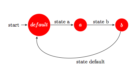
which would describe an abstract automaton with three distinct states, the starting state being always the state default.

Such a construct is a DFA and one could represent it graphically as a transition between states default, a and b (Figure 7). In this case, the automaton would loop between the three states, since on every state-transition, the state_entry event is raised in that particular state.

Our PGS exploits this concept since, as it happens, every single state in LSL can subscribe to global events and handle them internally. Taking the most basic example, the default Linden Hello World script that gets generated every time a new script is created, contains the following:

default
{
    state_entry()
    {
        llSay(0, "Hello, Avatar!");
    }
 
    touch_start(integer total_number)
    {
        llSay(0, "Touched.");
    }
}

which contains one state, the starting point of the automaton, default and two event handlers state_entry and touch_start. Similarly, all other states subscribe to events by simply mentioning the event handler in the body of the state:

default
{
    state_entry()
    {
        llSay(0, "Hello, Avatar!");
    }
 
    touch_start(integer total_number)
    {
        state nondefault;
    }
}
state nondefault
{
    state_entry()
    {
        llSay(0, "Goodbye, Avatar!");
    }
 
    touch_start(integer total_number)
    {
        state default;
    }
}

The usefulness follows, the script above is a simple flip-flop that when touched once, transitions from the default state to the user-named nondefault state. When touched again, it switches back to the default state. The usefulness derives from the fact that while the automaton is in the state nondefault, only that state is registered to all other global events. More concisely, only the current state gets updates from global events.

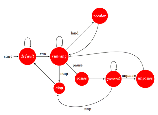
As the previous section mentioned, we use states in order to ensure that some operation is performed correctly. For example, the transitions:

running -> pause -> paused

and

paused -> unpause -> running

are used to ensure that the simulation stops by using an intermediary state. Our PGS accepts a paused state where all bats and moths, as well as the statistics overhead display freeze (including the elapsed time simulation). Since every flying object needs to be tracked, and since llRegionSay may prove unreliable, we temporarily switch to a pause state that proceeds to continuously rescans whether any object is still flying. If any object is still flying, it re-broadcasts the message (internally, this is done by calculating cumulative velocities). If it senses that no object is flying anymore, after some statistical heuristic, it jumps to the paused state. A similar procedure, yet not so complex, is done for dynamically changing environments while the PGS runs.

The main controller script for the PGS uses several stationary states where the automaton does not make transitions by itself. In the current PGS build, the default, running and paused are stationary states. If we take the case of the state paused, the only way to get out of that state is to execute an unpause command, leading to the unpause state and then back to the running state.

The automatons are taken further on the state machines page as well as an example thereof can be found on the Great Wanderer project page.

The PGS build has a few extensions which we would like to document here.

Real-Time data can be grabbed using the following scripts, courtesy of Wizardry and Steamworks. We have decided for a pie-chart because it allows us to see the distribution of genotypes. For example, on a neutral colored environment, one can immediately observe that the pie chart is symmetric indicating an equal and balanced distribution of all genotypes.

We are able to display more data by using the other chart types provided by the API but, for now, the pie chart will suffice.

• Based on Permanent Primitive URL, the LSL part of the system registers a permanent URL with tiny.cc and maps it to the URL generated in Second Life using llRequestURL. Since we like modularity, the script is integrated in the PGS statistics module which grabs all the important parameters from the rest of the build.

• The PHP script uses pChart to generate the chart, by pulling the data from the Permanent Primitive URL script in the PGS statistics module. It then computes the percentages by going through the data in order to display them on the chart.

pgs.php

<?php
 /*
    //////////////////////////////////////////////////////////
    // [K] Morgan LeFay - 2011, License: GPLv3              //
    // License at: http://www.gnu.org/licenses/gpl.html     //
    //////////////////////////////////////////////////////////
 
    PGS ONE: Example PGS graphing script which dynamically
    generates graphs based on the current genotypes in the PGS                        
 
 */
 
 // Standard inclusions   
 include("pChart/pData.class");
 include("pChart/pChart.class");
 
 $pgs = file_get_contents('http://tiny.cc/pgs_one');
 $dataGenotypeName = array_splice(str_getcsv($pgs), 2, 4);
 //DEBUG: Show genotype names as array, needs the image renderer
 //to be disabled in order not to clash with the Content-Type
 //print_r($dataGenotypeName);
 $dataGenotypeValue = array_splice(str_getcsv($pgs), 10, 4);
 //DEBUG: Show the genotype values.
 //print_r($dataGenotypeValue);
 
 // Sum-up genotype count so we have a total number of creatures
 // and later use that to calculate percentages.
 $totalGenotypes = 0;
 foreach ($dataGenotypeValue as $key => $value) {
   $totalGenotypes += $value;
 }
 
 // Finally calculate the percentages which will show the 
 // distribution of genotypes. Computed as:
 // 100 * some_genotype / total_number_of_genotypes
 $dataValues = array();
 foreach ($dataGenotypeValue as $key => $value) {
   array_push($dataValues, intval(100 * $value / $totalGenotypes));
 }
 //DEBUG: Debug the percentages to make sure we did that correctly
 //print_r($dataValues);
 
 // Dataset definition 
 $DataSet = new pData;
 $DataSet->AddPoint($dataValues,"Serie1");
 $DataSet->AddPoint($dataGenotypeName,"Serie2");
 $DataSet->AddAllSeries();
 $DataSet->SetAbsciseLabelSerie("Serie2");
 
 // Initialise the graph
 $PGS_ONE = new pChart(420,250);
 $PGS_ONE->drawFilledRoundedRectangle(7,7,413,243,5,240,240,240);
 $PGS_ONE->drawRoundedRectangle(5,5,415,245,5,230,230,230);
 $PGS_ONE->createColorGradientPalette(195,204,56,223,110,41,5);
 
 // Draw the pie chart
 $PGS_ONE->setFontProperties("Fonts/tahoma.ttf",8);
 $PGS_ONE->AntialiasQuality = 8;
 $PGS_ONE->drawPieGraph($DataSet->GetData(),$DataSet->GetDataDescription(),180,130,110,PIE_PERCENTAGE_LABEL,FALSE,50,20,5);
 $PGS_ONE->drawPieLegend(350,15,$DataSet->GetData(),$DataSet->GetDataDescription(),250,250,250);
 
 // Write the title
 $PGS_ONE->setFontProperties("Fonts/MankSans.ttf",10);
 $PGS_ONE->drawTitle(10,20,"PGS ONE",100,100,100);
 
 // Set content-type to PNG. Disable this for previous  DEBUG instances.
 header('Content-Type: image/png');
 // Render! Disable this for the previous DEBUG instances.
 $PGS_ONE->Stroke();
 
?>

• The html part, is a jQuery wrapper that reloads the chart every few seconds. It is based originally on a jQuery div refresh which we converted to refresh an image tag instead.

pgs.html

<html>
<head>
<!-- This should be replaced with the latest copy of jQuery -->
<script src="http://code.jquery.com/jquery-latest.js"></script>
<script>
 $(document).ready(function() {
         $("#responsecontainer").load("pgs.php");
   var refreshId = setInterval(function() {
      $("#pgs").attr("src", "pgs.php?d="+ new Date().getTime());
   }, 5000);
   $.ajaxSetup({ cache: false });
});
</script>
</head>
<body>
<img id="pgs" src="pgs.php">
</body>
</html>

The jQuery appends a date and changes the src attribute of the img tag. This is done on purpose in order to avoid image-cachers.

Alternatively, if you do not wish to rely on tiny.cc - which may be a bad choice, you can use the same Permanent Primitive URL script and amend the PHP script so use a local database to update the URL:

pgs_graph.php

<?php
 /*
    //////////////////////////////////////////////////////////
    // [K] Morgan LeFay - 2011, License: GPLv3              //
    // License at: http://www.gnu.org/licenses/gpl.html     //
    //////////////////////////////////////////////////////////
 
    PGS ONE: Example PGS graphing script which dynamically
    generates graphs based on the current genotypes in the PGS                        
 
 */
 
 // Standard inclusions   
 include("pChart/pData.class");
 include("pChart/pChart.class");
 
 // Insert simulator URL if the user has authed.
 if(isset($_GET['login']) && isset($_GET['apiKey'])) {
  if($_GET['login'] == 'loginUSER' && $_GET['apiKey'] == '9F2B82C4-F820-430B-8AB5-4A7861F9C0E5') {
   if(isset($_GET['longUrl']) && isset($_GET['shortUrl'])) {
    $longURL = $_GET['longUrl'];
    $shortURL = $_GET['shortUrl'];
    $link = mysql_connect('DATABASE_HOST', 'DATABASE_USERNAME', 'DATABASE_PASSWORD');
    if(!$link) {
     print 'Sorry, a database connection could not be established.';
     return;
    }
    mysql_select_db('DATABASE_NAME', $link);
    $query = sprintf("DELETE FROM pgs_url WHERE short_url='%s'", 
     mysql_real_escape_string($shortURL, $link));
 
    mysql_query('LOCK TABLES pgs_url WRITE', $link);
    $queryResult = mysql_query($query, $link);
    mysql_query('UNLOCK TABLES', $link);
 
    $query = sprintf("INSERT INTO pgs_url (sim_url, short_url) VALUES ('%s', '%s')",
     mysql_real_escape_string($longURL, $link),
 
    mysql_query('LOCK TABLES pgs_url WRITE', $link);
    $queryResult = mysql_query($query, $link);
    mysql_query('UNLOCK TABLES', $link);
    mysql_close($link);
   }
  }
 }
 
 // Connect to database and fetch simulator URL based on short url.
 $link = mysql_connect('DATABASE_HOST', 'DATABASE_USERNAME', 'DATABASE_PASSWORD'); 
 if(!$link) {
   print 'Sorry, a database connection could not be established.';
   return;
 }
 mysql_select_db('DATABASE_NAME', $link);
 $query = sprintf("SELECT sim_url FROM pgs_url WHERE short_url='%s'",
  mysql_real_escape_string('pgs_one', $link));
 $queryResult = mysql_query($query, $link);
 $longURL = mysql_result($queryResult, 0, 'sim_url');
 $shortURL = mysql_result($queryResult, 0, 'short_url');
 mysql_close($link);
 
 //DEBUG: Check if the simulator URL is correct.
 //print 'URL: '.$longURL;
 
 $pgs = file_get_contents($longURL);
 $dataGenotypeName = array_splice(str_getcsv($pgs), 2, 4);
 //DEBUG: Show genotype names as array, needs the image renderer
 //to be disabled in order not to clash with the Content-Type
 //print_r($dataGenotypeName);
 $dataGenotypeValue = array_splice(str_getcsv($pgs), 10, 4);
 //DEBUG: Show the genotype values.
 //print_r($dataGenotypeValue);
 
 // Sum-up genotype count so we have a total number of creatures
 // and later use that to calculate percentages.
 $totalGenotypes = 0;
 foreach ($dataGenotypeValue as $key => $value) {
   $totalGenotypes += $value;
 }
 
 // Finally calculate the percentages which will show the 
 // distribution of genotypes. Computed as:
 // 100 * some_genotype / total_number_of_genotypes
 $dataValues = array();
 foreach ($dataGenotypeValue as $key => $value) {
   array_push($dataValues, intval(100 * $value / $totalGenotypes));
 }
 //DEBUG: Debug the percentages to make sure we did that correctly
 //print_r($dataValues);
 
 // Dataset definition 
 $DataSet = new pData;
 $DataSet->AddPoint($dataValues,"Serie1");
 $DataSet->AddPoint($dataGenotypeName,"Serie2");
 $DataSet->AddAllSeries();
 $DataSet->SetAbsciseLabelSerie("Serie2");
 
 // Initialise the graph
 $PGS_ONE = new pChart(420,250);
 $PGS_ONE->drawFilledRoundedRectangle(7,7,413,243,5,240,240,240);
 $PGS_ONE->drawRoundedRectangle(5,5,415,245,5,230,230,230);
 $PGS_ONE->createColorGradientPalette(195,204,56,223,110,41,5);
 
 // Draw the pie chart
 $PGS_ONE->setFontProperties("Fonts/tahoma.ttf",8);
 $PGS_ONE->AntialiasQuality = 8;
 $PGS_ONE->drawPieGraph($DataSet->GetData(),$DataSet->GetDataDescription(),180,130,110,PIE_PERCENTAGE_LABEL,FALSE,50,20,5);
 $PGS_ONE->drawPieLegend(350,15,$DataSet->GetData(),$DataSet->GetDataDescription(),250,250,250);
 
 // Write the title
 $PGS_ONE->setFontProperties("Fonts/MankSans.ttf",10);
 $PGS_ONE->drawTitle(10,20,"PGS ONE",100,100,100);
 
 // Set content-type to PNG. Disable this for previous  DEBUG instances.
 header('Content-Type: image/png');
 // Render! Disable this for the previous DEBUG instances.
 $PGS_ONE->Stroke();
 
?>

You will also need to do the following:

• create a new database, referenced in the script as DATABASE_NAME.
• change DATABASE_NAME, DATABASE_USERNAME, DATABASE_PASSWORD and DATABASE_HOST to their corresponding values.
• create a new table, with one field called sim_url and the other short_url.
• alter the Permanent Primitive URL and replace all instances of http://tiny.cc/ with the corresponding path to this PHP script.

This essentially emulates the service provided by tiny.cc so that just the URL must be changed in the Permanent Primitive URL.

So far, the build finds itself in a working-beta phase. That is, the PGS both operable and usable. However, we aim to optimize some parts of the scripts. For example, the Wanderer script is taken as it is and modified accordingly to capture messages for the origin position from where all coordinates are generated. The Wanderer script contains multiple coordinate generation shapes such as lower-hemisphere, squares, and so on, which are not needed for the PGS itself and can be factored out. Furthermore, given that we just use one single geometric body or shape per creature, it would be feasible to inline most of the Wanderer coordinate generation function.

Further enhancements and small optimizations are also possible however, at some point this build will become a part of the Science Grid and used by the VIBE group for teaching. Since the Science Grid uses the OpenSIM as a platform, we are hesitant to optimize any further than that because in its current state the OpenSIM has various levels of implementation for the LSL functions we use. For one, the Wanderer script, in its non-altered verbatim state as it is to be found on this wiki is not fully compatible with the OpenSIM. Physics are lackey as well in the OpenSIM implementation, varying between various physics engines.