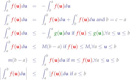
Definite Integral

A definite integral is written $\int_{a}^{b}f(x)dx$ and are commonly used to find the area between the graph of a function and the x-axis.

Example

$\begin{eqnarray*} \int_{2}^{5}x^{2}dx &=& \frac{1}{3}x^{3}\biggr\vert_{2}^{5} & \\ &=& \frac{1}{3}(5)^{3}-\frac{1}{3}(2)^{3} \end{eqnarray*}$

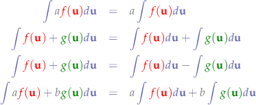
Integrals of Common Functions

${\color{gray}a},{\color{gray}b},{\color{gray}c}$ are constants, $\bf{u}$ is a variable and ${\color{red}f}$ , ${\color{green}g}$ are functions.

$\begin{eqnarray*} \int{{\color{gray}a}{\color{red}{\color{red}f({\bf{u}})}}d{\bf{u}}} &=& {\color{gray}a}\int{{\color{red}{\color{red}f({\bf{u}})}}d{\bf{u}}} & \\ \int{{\color{red}{\color{red}f({\bf{u}})}}+{\color{green}g({\bf{u}})}}d{\bf{u}} &=& \int{{\color{red}{\color{red}f({\bf{u}})}}}d{\bf{u}} + \int{{\color{green}g({\bf{u}})}}d{\bf{u}} & \\ \int{{\color{red}{\color{red}f({\bf{u}})}}+{\color{green}g({\bf{u}})}}d{\bf{u}} &=& \int{{\color{red}{\color{red}f({\bf{u}})}}}d{\bf{u}} - \int{{\color{green}g({\bf{u}})}}d{\bf{u}} & \\ \int{{\color{gray}a}{\color{red}{\color{red}f({\bf{u}})}}+{\color{gray}b}{\color{green}g({\bf{u}})}}d{\bf{u}} &=& {\color{gray}a}\int{{\color{red}{\color{red}f({\bf{u}})}}}d{\bf{u}} + {\color{gray}b}\int{{\color{green}g({\bf{u}})}}d{\bf{u}} & \\ \end{eqnarray*}$

$\begin{eqnarray*} \int{{\bf{u}}d{\bf{v}}} &=& {\bf{u}}{\bf{v}} - \int{{\bf{v}}d{\bf{u}}} \end{eqnarray*}$

$\begin{eqnarray*} \int_{{\color{gray}a}}^{{\color{gray}b}}{\color{red}{\color{red}f({\bf{u}})}}d{\bf{u}} &=& -\int_{{\color{gray}b}}^{{\color{gray}a}}{\color{red}{\color{red}f({\bf{u}})}}d{\bf{u}} & \\ \int_{{\color{gray}a}}^{{\color{gray}c}}{\color{red}{\color{red}f({\bf{u}})}}d{\bf{u}} &=& \int_{{\color{gray}a}}^{{\color{gray}b}}{\color{red}{\color{red}f({\bf{u}})}}d{\bf{u}} + \int_{{\color{gray}b}}^{{\color{gray}c}}{\color{red}{\color{red}f({\bf{u}})}}d{\bf{u}} \text{ and } {\color{gray}b} = {\color{gray}c}-{\color{gray}a} & \\ \int_{{\color{gray}a}}^{{\color{gray}b}}{\color{red}{\color{red}f({\bf{u}})}}d{\bf{u}} &\le& -\int_{{\color{gray}b}}^{{\color{gray}a}}{\color{green}g({\bf{u}})}d{\bf{u}} \text{ if } {\color{red}{\color{red}f({\bf{u}})}} \le {\color{green}g({\bf{u}})} \text{,} \forall {\color{gray}a} \le {\bf{u}} \le {\color{gray}b} & \\ \int_{{\color{gray}a}}^{{\color{gray}b}}{\color{red}{\color{red}f({\bf{u}})}}d{\bf{u}} &\le& M({\color{gray}b}-{\color{gray}a}) \text{ if } {\color{red}{\color{red}f({\bf{u}})}} \le M \text{,} \forall {\color{gray}a} \le {\bf{u}} \le {\color{gray}b} & \\ m({\color{gray}b}-{\color{gray}a}) &\le& \int_{{\color{gray}a}}^{{\color{gray}b}}{\color{red}{\color{red}f({\bf{u}})}}d{\bf{u}} \text{ if } m \le {\color{red}{\color{red}f({\bf{u}})}} \text{,} \forall {\color{gray}a} \le {\bf{u}} \le {\color{gray}b} & \\ \biggr\vert \int_{{\color{gray}a}}^{{\color{gray}b}}{\color{red}f({\bf{u}})}d{\bf{u}} \biggr\vert&\le& \int_{{\color{gray}a}}^{{\color{gray}b}}\vert {\color{red}{\color{red}f({\bf{u}})}} \vert d{\bf{u}} \text{ if } {\color{gray}a} \le {\color{gray}b} \end{eqnarray*}$

Differentiating Integrals

Differentiation is the symmetric operation of integrating:

$\begin{eqnarray*} \frac{d}{d{\bf{x}}}\biggr{[}\int {\bf{x}}d{\bf{x}}\biggr{]} &=& {\bf{x}} \end{eqnarray*}$

Convolution Integral

The convolution of two functions (over the same variable, e.g. $f_{1}{t}$ and $f_{2}{t}$ ) is an operation that produces a separate third function that describes how the first function modifies the second one. Conversely, the resulting function can also be used to describe how the second function modifies the fist function.

The convolution of two functions is denoted with the $*$ operator and written as:

$\begin{eqnarray*} f_{1}(x) * f_{2}(x) &=& \int_{-\infty}^{\infty} f_{1}{\tau} \cdot f_{2}(t-\tau) d\tau \end{eqnarray*}$

where $\tau$ is a dummy variable.

Here is an example of the convolution of two square pulses $f(t)$ and $g(t-\tau)$ :

resulting in $(f*g)(t)$ .

Properties

Commutativity.

$\begin{eqnarray*} f_{1}(t) * f_{2}(t) &=& f_{2}(t) * f_{1}(t) \end{eqnarray*}$

Distributivity.

$\begin{eqnarray*} f_{1}(t) * (f_{2}(t) + f_{3}(t)) &=& f_{1}(t) * f_{2}(t) + f_{1}(t) * f_{3}(t) \end{eqnarray*}$

Shift

If:

$\begin{eqnarray*} f_{1}(t) * f_{2}(t) &=& c(t) \end{eqnarray*}$

then:

$\begin{eqnarray*} f_{1}(t-T_{1}) * f_{2}(t-T_{2}) &=& c(t-T_{1}-T_{2}) \end{eqnarray*}$

Convolution with an impulse results in the original function (neutral element).

$\begin{eqnarray*} f(t) * \sigma(t) &=& f(t) \end{eqnarray*}$

where $\sigma(t)$ is the unit impulse.

Width: the convolution of a signal of duration $T_{1}$ and a signal of duration $T_{2}$ will result in a signal of duration $T_{3} = T_{1} + T_{2}$ .

Convolution Integral and Circuits

Most electrical circuits are designed to be linear, time-invariant systems (LTI) meaning that the magnitude of a circuit's output signal is a scaled version of the input signal's magnitude. Furthermore, and LTI system that is given two independent signal sources will output the sum of the scaled versions of each signal. Given a function $x_{1}(t)$ that causes an LTI system to output $y_{1}(t)$ , then:

$\begin{eqnarray*} a_{1} \cdot x_{1}(t) &\mapsto& a_{1} \cdot y_{1}(t) \end{eqnarray*}$

where $a_{1}$ is a multiplicative constant. Given a number of independent signal sources, this gives rise to the concept of signal superposition which allows us to say:

$\begin{eqnarray*} a_{1} \cdot x_{1}(t) + a_{2} \cdot x_{2}(t) + \ldots + a_{n} \cdot x_{n}(t) &\mapsto& a_{1} \cdot y_{1}(t) + a_{2} \cdot y_{2}(t) + \ldots + a_{n} \cdot y_{n}(t) \end{eqnarray*}$

A time-invariant system means it does not matter when the input signal is applied - a specific input signal will always result in the same output signal for a given LTI system. The time-invariance can be expressed as:

$\begin{eqnarray*} x_{1}(t) \mapsto y_{1}(t) &\Leftrightarrow& x_{1}(t+\tau) \mapsto y_{1}(t+\tau) \end{eqnarray*}$

where $\tau$ can be viewed as a time delay when dealing with signals in time (i.e. "time-domain signals"). Indirectly, this concept also signifies than an output signal cannot contain frequency components not inherent in the input signal (causality).

The vast majority of circuits are LTI systems, each with a specific impulse response. The "impulse response" of a system is a system's output when its input is fed with an impulse signal - a signal of a brief duration. An example of an "impulse signal" would be a lighting bolt or any form of ESD (electro-static discharge). Any voltage or current that spikes in magnitude for a relatively short period of time may be viewed as an impulse signal. The impulse response of a circuit will always be a time-domain signal and exists because no signal can propagate through a circuit will always be a time-domain signal, and exists because no signal can propagate through a circuit in zero time; each individual electron involved can only move so quickly through each component. Real-world electronic LTI systems exhibit an impulse response that consists of an initial spike in magnitude, followed by an everlasting and ever-decreasing exponential relationship in signal magnitude.

The integral of the impulse response and the input square wave stepped through time can be observed in the image above. The convolution equation is seen as the operation is done with respect to $\tau$ . In reality, we are taking an input signal, flipping it vertically through the origin and determining whether the what the integral is for each value of $\tau$ which represents in this case a delay through time. Since the output of any LTI system is non-casual (it cannot exist until the signal that excites the output has seen applied), we must step through time to see how each impulse signal of the input affects the LTI system's impulse response - again, achieved by stepping through $\tau$ - the "time-delay" dummy variable.

Example

For an LTI system with an impulse response of $h(t)=e^{-2t}u(t)$ , calculate the output $y(t)$ given the input of $f(t) = e^{-t}u(t)$ .

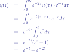
Using the convolution integral, we have to solve:

$\begin{eqnarray*} y(t)&=&h(t) * f(t) = \\ &=&\int_{0}^{\infty}h(\tau)*f(t-\tau)d\tau \end{eqnarray*}$

It only makes sense to integrate between $0$ and $+\infty$ because at $t=0$ the signal is applied and both $h(t)$ and $f(t)$ will have zero magnitude at any time $t < 0$ .

Now we can calculate:

$\begin{eqnarray*} y(t) &=& \int_{0}^{\infty} e^{-2\tau} u(\tau) \cdot e^{-\tau} d\tau \\ &=& \int_{0}^{t} e^{-2(t-\tau)} \cdot e^{-\tau} d\tau \\ &=& e^{-2t} \int_{0}^{t} e^{\tau} d\tau \\ &=& e^{-2t} (e^{t} - 1) \\ &=& e^{-t} - e^{-2t} \end{eqnarray*}$